


1. Introduction
Electroplating is a surface treatment method widely used in manufacturing processes of electronic parts such as displays, mobile phones, semiconductors, etc. [1–3]. Deposition thickness uniformity is critical to improve product quality and productivity for these applications [4,5]. Because electroplating processes are affected by many parameters such as pH, temperature, current density, plating time, metal ions, concentration, agitation [6], and experimental approaches are difficult to estimate the effects of these parameters. So, many studies using simulation have been conducted for efficient studies [1–3,7–12].
Currently, the electroplating simulation method mainly used is to calculate the secondary current distribution considering the electric field distribution and the overvoltage depending on the shape of the plating system [3,7,9]. This method is widely used because it is possible to simulate complex shapes [3,7,9]. The method is based on the assumption that the agitation of the electrolyte is sufficiently strong to achieve complete mixing. However, in many processes, the flow may not be uniform and not enough to make complete mixing, so unevenness of the deposition thickness appears because of non-uniform fluid flow [2].
In order to overcome this limitation, studies are underway to calculate the tertiary current distribution with additional consideration of the mass transfer effect due to the flow [1,2,8]. Low et al. [1] and Ji et al. [2] obtain the thickness of the diffusion layer through empirical equations. Inside the layer, electroplating is calculated considering the concentration gradient, and the outside is treated as a bulk having a constant concentration. Tong [8] calculated the concentration distribution considering the fluid flow. In this way, various results such as current density, voltage, and concentration distribution can be obtained according to the stirring speed and position.
However, three-dimensional tertiary current distribution study is limited in practical applications because the simulation model is complicated and needs very long calculation time [11,12]. So this approach is limited to two-dimensional studies of simple shapes such as a rotating cylinder electrode (RCE) [1] or rotating disc electrode (RDE) [2,8].
In the present study, we propose a new electroplating simulation method that can be applied to complex shapes and analyse the effect of flow.
2. Experimental
2.1. Outlines of the model
In this study, polarization curves are used to consider the effect of flow. The polarization curve is a graph which shows the relationship between the current density and the overvoltage, and it includes various electrochemical characteristics of the plating solution [13]. Thus, polarization curves can be used directly as boundary conditions for electroplating calculations [3], or Tafel slope and exchange current density obtained through them can be used as variables [1,2,8]. In particular, the effect of flow is also expressed in the polarization curves, and it has been studied through experiments and calculations [14–17]. Also, the polarization curves varying with the flow rate can be obtained from the results of the calculations by the tertiary current distribution method [1,8].
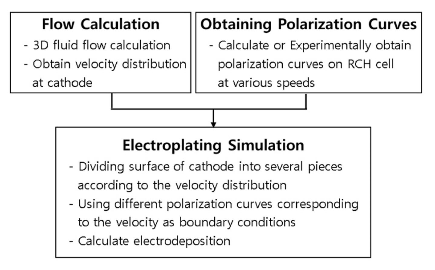
The limitation of the use of the polarization curve is that the previous studies use one polarization curve for plane even though the fluid conditions are not uniform on the plane. The novelty of the present study is that multiple polarization curves can be used for one plane. The method is divided into three stages as shown in Fig. 1. First, a three-dimensional flow analysis is performed on the plating system to obtain flow distribution, in particular, flow velocity distribution information on the surface of the cathode. Next, polarization curves at various flow rates are calculated or experimentally obtained. Finally, the surface of the cathode is divided into several parts according to the flow rate, and electroplating calculation is performed while using different polarization curves corresponding to the flow rate as boundary conditions.
2.2. Flow calculation
We calculate fluid flow behavior of electrolyte using flow and standard k-e turbulence modules of a commercial program CFD-ACE+ with the following governing equations.
where ρ is the density; t is the time; V is the flow velocity vector field; u, v and w are the fluid velocity in the x, y, z-direction; p is the pressure; μ is dynamic viscosity; SMx, SMy and SMz are the rate of increase of x, y, z-momentum due to sources, respectively [18].
A magnetic stirrer generates the flow, and it is calculated using a two-blade fan model [18]. This model does not make a complicated grid system to simulate the moving parts of the stirrer and without having to model the transient effects of the rotating stirrer. Instead, it predicts the time-averaged force applied to the fluid based on information such as the geometrical parameters (location, size, etc.) and the rotational speed of the stirrer and the local flow conditions.
Calculation was performed on the flow of the fluid in the bath. The fluid used in this calculation is water, the density is 997 kg/m3 and the kinematic viscosity is 1.09×10⁻⁶ m2/s. The electrodes treated as blocks to prevent flow. The grid was composed of an unstructured of 882192 cells. The walls of electrode and bath are zero flow and no-slip wall condition, and the fan is used as a flow source.
The effects of electromagnetic field on fluid flow is small because the electroplating currents and electric conductivity of electrolyte are small. So the electromagnetic field is not taken into consideration for fluid flow calculation. Also, chemical reactions and heat transfer were not considered because the reactions for copper plating occurs just near the electrode so the effects of the reactions on fluid flow can be negligible. The stirring behavior was calculated by the fan blade model of CFD-ACE+ and we assumed steady state without considering the vortex.
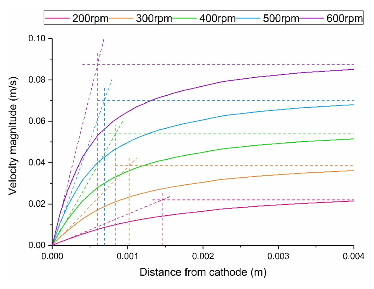
The fluid flow distributions on the cathode surface which actually affect the electroplating are used. The value of the distance from the surface of the cathode is determined through the velocity boundary layer. The thickness of the boundary layer is determined by using tangent line to the initial slope of the velocity distribution in the vertical direction of the cathode as shown in Fig. 2. The distance from the surface to the position where the value of the tangent line is equal to the bulk value is used as the value of boundary thickness. Table 1 shows the values of the boundary layer at different rotation rate.
2.3. Obtaining Polarization curves
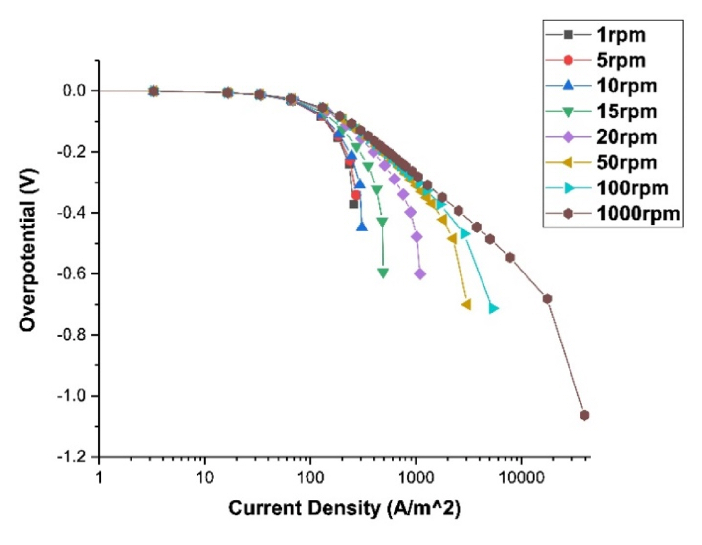
The polarization curves for use as boundary conditions for electroplating calculations can be obtained from the experiments or calculations. We need polarization curves in different flow conditions. In the present study, we calculate polarization curves at the RCH (Rotating cylinder Hull) cell [19] using the commercial program CFD-ACE+. We use a 2D axisymmetric mesh to calculate the tertiary current distribution [18] while varying the voltage (or current density) from 0.0001 to 100 V (0.01 to 10000 A/m2). In this way, the current density and the overvoltage on the cathode surface are obtained, and one point is obtained for each of these calculations. Then the polarization curve is acquired by connecting these points. Also, the polarization curves are obtained by changing the rotation speed of the cathode of the RCH cell from 1 to 1000 rpm.
2.4. Electroplating calculation
Electroplating calculations are carried out using a program developed using the model of Mehdizadeh et al. [20] and Oh et al. [10]. The potential distribution in the plating bath is calculated by the Laplace equation, and in particular, the potential at the cathode is calculated taking into account the surface overvoltage and the concentration overvoltage. Through the finite element method, the overvoltage is obtained by the under-relaxation method, and the convergence solution is obtained by repeating the process of solving the Laplace equation using it [10, 20]. Here, the cathode surface is divided into several sections so that different polarization curves are used as boundary conditions on each section.
Based on the calculated velocities of each section, one appropriate polarization curve is selected for each section. For comparing the velocities of RCH cell, angular velocities are converted to linear velocities by the equation v = r × w. For the calculation, eight polarization curves are used at 1, 5, 10, 15, 20, 50, 100, and 1000 rpm. The intermediate values are used by interpolation. The electroplating calculations can obtain the deposition thickness, voltage, and current density distribution for 0.5M CuSO4, and 1M H2SO4 plating solution is subjected to a current of 1.2A at room temperature for 45 minutes. The specific physical properties of the plating solution are shown in Table 2.
2.5. Experimental techniques for verification of the model
We conduct three experiments, one is for verification of flow calculations, another for verification of polarization curves, and the other is for verification of electroplating calculation. The plating bath used in the electroplating experiments is made of a transparent acrylic cube with a width of 140 mm and a height of 140 mm as shown in Fig. 3. A brass anode of 150 mm (L) × 50 mm (W) × 2 mm (t) and a SUS cathode of 150 mm (L) × 60 mm (W) × 0.5 mm (t) are installed at both ends. The cathode is masked, so plated only in a region of 60 mm × 40 mm.
In order to verify the flow analysis, a Particle Image Velocimetry (PIV) experiment is conducted to measure the flow using a laser. Using the system with the same structure of the electroplating experiment, we use water instead of the plating solution, add particles for laser measurement, and conduct measurements while changing the stirring speed.
The PIV should be measured with the camera in the direction perpendicular to the surface to be illuminated through the laser. It is difficult to directly measure the surface of the cathode because the anode and the cathode are facing each other, so bulk velocity profiles are measured and compared to the calculated values. 10000 images are obtained for 250 fps × 40 sec in the vertical direction at the height of 80 mm, and a two-dimensional velocity distribution is obtained by averaging them.
Experiments for the verification of the calculated polarization curves are carried out in an RCH cell. In the same plating solution as in the electroplating experiment, the current density change is measured with PARSTAT 2273 potentiostat using the Ag / AgCl reference electrode while changing the rotation speed of the cathode from 1 to 1000 rpm.
Electroplating experiments are conducted under the same conditions as the calculation. The deposition thickness is measured for a total of 96 points of 12 points × 8 points using a Fischerscope XRF (X-Ray Fluorescence).
3. Results and Discussion
3.1. Results of fluid flow by numerical simulations and experiments
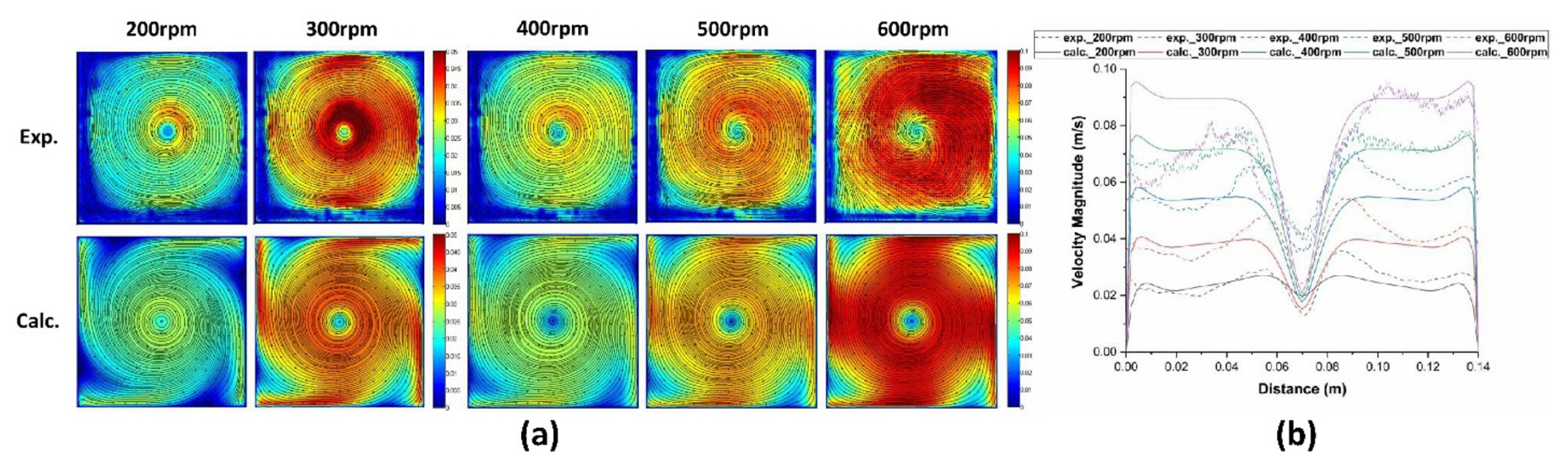
Because the present model starts from the calculated fluid flow profiles, verification of the results of fluid flow simulation is crucial. So fluid flow occurred by a stirrer was simulated and compared the results to the those of experiments. In order to simulate agitation using a stirrer, a fan model was used. In this case, a correction factor by the empirical equation is needed [18], and it is obtained through comparison with experimental data. The velocity distribution at the 80mm height section was measured using PIV and compared with the calculated values. Two-dimensional velocity streamlines of a cross section at the 80 mm height at different rotation rates are shown in Fig. 4(a). The distribution of the flow velocity shows that large vortex was formed at the center and the velocity of center is very low. The pattern becomes extending like a windmill.
The line profiles of velocity along a line of the plane obtained by experiments and calculations are compared in Fig. 4(b). As shown in the figure, the profiles and values of velocity are similar each other.
From the comparison, it can be seen that the range of the velocity values of the results obtained by experiments and numerical calculations are similar for each stirring speeds. So, the reliability of the calculation can be confirmed through the above results.
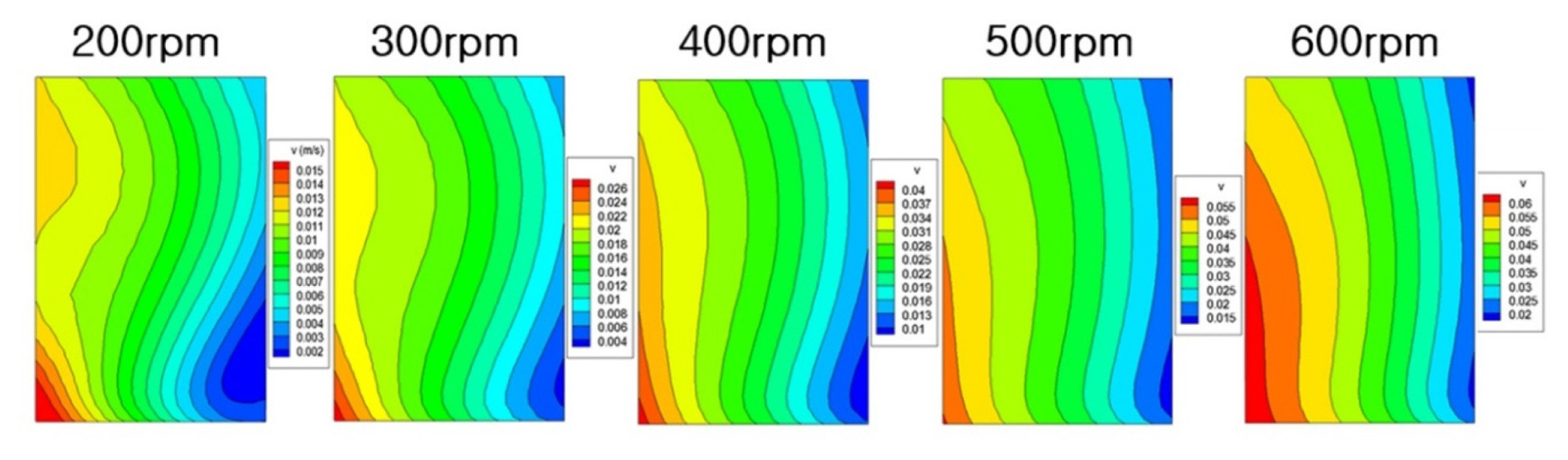
Through the flow analysis, the flow velocity distribution on the surface of the cathode according to the stirring speed was obtained as shown in Fig. 5. As rotation rates are increased, the values of velocity increase. On the other hand, the profiles are similar at different rotation rates. And velocities of left part are greater than right part. The purpose of the present study is to calculate the effects of the velocity magnitudes and profiles on the deposition behavior on the electrode.
3.2. Obtaining polarization curves
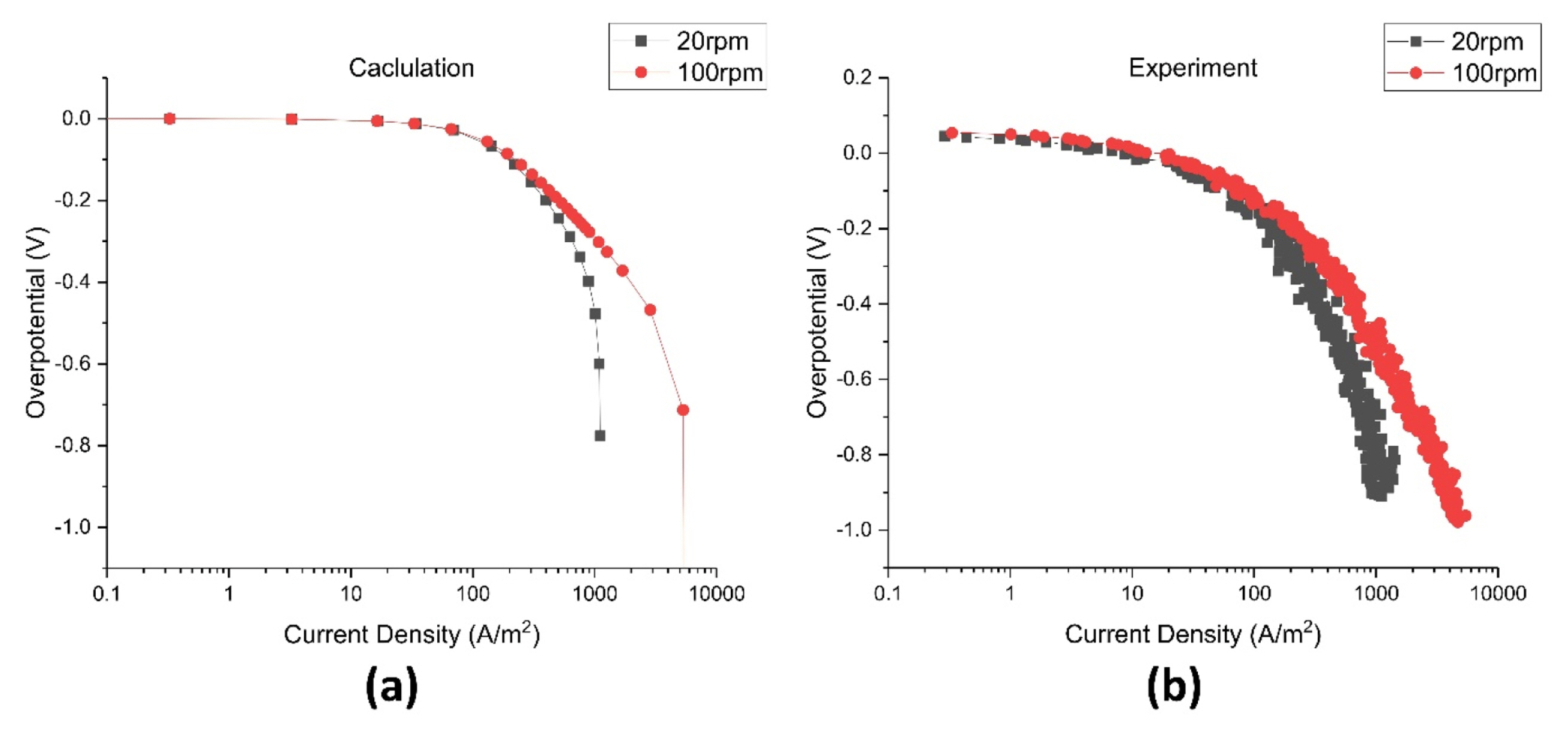
Because the polarization curves at different fluid velocities were necessary for calculating electrodeposition behavior, polarization curves were calculated at different velocities. Fig. 6. shows the polarization curves which obtained at 1, 5, 10, 15, 20, 50, 100, and 1000 rpm rotating speed in RCH cell, and it can be seen that as the speed increases, the limit current increases and moves to the right. Experiments for obtaining polarization curves are also conducted to verify the calculations. The experiment and calculation are compared at 20, 100 rpm as shown in Fig. 7.
3.3. Calculation the thickness of electroplating deposition
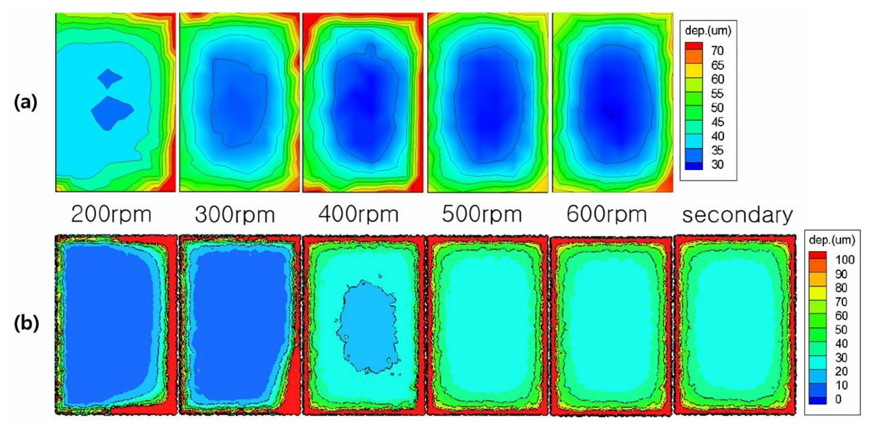
Figure 8(a) shows experimental results of the deposition thickness of the electroplating system according to stirring speed 200~600 rpm. The results showed that the thickness of the deposition layer on the outside regions of the cathode is thicker than that on the inside region. This uneven thickness distribution appears at all rotation rates. The experiments showed another uneven distribution which depended on fluid velocity. At low rotation rates, the thickness of left side was thinner than that of right side. However, as rotation rates increase, the thickness of both side became similar.
These thickness behavior were well simulated by the present model as shown in Fig. 8(b). The calculation results also showed that thickness of outside region was thicker than that of inside region. Thickness of left side was thinner than that of right side at low rotation rates and thickness of both side became similar as rotation rates were increasing. All behaviors were well matched with experimental results.
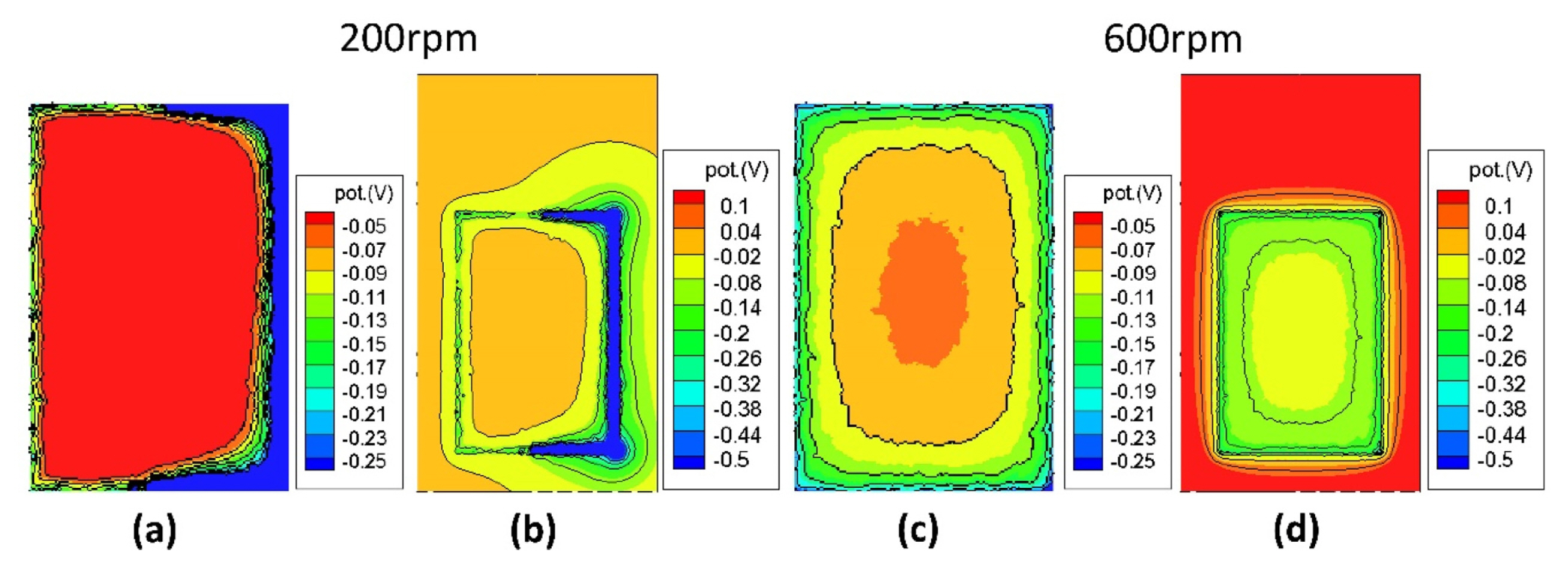
Analysis of the calculation results showed that the fast deposition rates of outside region is caused by the high concentration of current density at the edge region [13]. And we can consider the cause of the difference between left side and right side through the electric potential distribution. Figure 9 shows the calculation results of potential distribution of the plating area and cathode at low rotation rate (200 rpm) and high rotation rate (600 rpm). We can see that the potential distribution also basically show that the potentials are concentrated outside the plating area. In the case of high rotation rate, it represents a symmetrical pattern in which the potential gradually increases from the edge of the plating area inward and outward. At low rotating rate with insufficient agitation, however, a lower potential is applied on the relatively slower right side. This asymmetrical distribution results in a non-uniform deposition thickness distribution. On the other hand, compared to velocity distribution in Fig. 5, it can be seen that faster side is thinner than slow side. This means that the deposition rate is rather slow due to strong convection of flow [2, 21]. Also, the non-uniformity of the deposition thickness is alleviated as the rotation speed is increased, and the influence of the agitation no longer occurs when the rotation speed is higher than a certain value [10].
The last figure of Fig. 8(b) showed the results of most popular calculation model (usually called by “secondary calculation”) for electrodeposition, the result was nearly same to the high rotation rates. This model can’t explain or reproduce the results of low rotation rates because the model is based on the assumption that fluid flow is sufficient.
Figure 8 showed that the present model can consider the effects of fluid flow on the electro-deposition behavior and the calculation results were well matched to the experimental results. So the present model should be very useful to simulate practical electro-deposition processes in which fluid flow is not sufficient so the deposition behaviors are affected by fluid flow.
4. Summary
We developed a new simulation model for three-dimensional electroplating system with non-uniform fluid flow. The model can predict the effects of fluid flow on the film thickness of electrodeposition process. To achieve this purpose, this model combines fluid flow simulation, polarization curve calculation and electrochemical simulation with electroplating kinetics.
This model is composed of three parts. One is calculating fluid flow, and the second is calculating polarization curves. Lastly, the two results are merged into the electroplating calculation model to estimate the effects of fluid flow on the uniformity of the thickness of electrodeposition on the electrode.
The ability of prediction of the model were verified by comparing calculated results with experimental results of fluid flow, polarization curves and electrodeposition.
The deposition thickness showed non-uniform distributions in experiments with plane electrode. At first the thickness of edge area is thicker than that of inner region and the profiles show symmetric profiles at high rotation rates. And then, the thicknesses of left side are thinner than those of right side when rotation rates were low.
The present model showed that the first phenomenon of thick deposition layer in the outer region is caused by the distribution of current intensity and the second behavior of different thickness of the left side and right side at low rotation rates is explained by the potential distribution and the velocity distribution. These results showed the necessary of the present model to consider the effects of fluid flow on the deposition behavior.