


1. Introduction
In PEMFC assembly, it consists of the dielectric membrane-Nafion, gas diffusion layers, electrolyte, electrodes, catalyst and gas sources (i.e. hydrogen and oxygen gases). The membrane requires sufficient liquid water in operation. Thus, the usual operation temperature is below 90┬░C which preventing a high evaporation rate in the system. In a complete electrical circuit, the electrons move from anode to cathode through the wires and electrical resistances. Simultaneously, the electrons move within the PEMFC assembly from cathode to anode. Commonly, the working principle of PEMFC is explained from the perspective of ions transport. Herein, this paragraph explains the working principle from the perspective of charge carriers as it requires far less energy for the electrons to move from an ion to another ion. It is a similar concept to explain the movement of charge carriers in a transistor. The motion of electrons relative to the electrolytes (from the cathode to the anode) is as if the protons (hydrogen ions) travel in the opposite direction. During the operation, the anode side, which separated by the layers receives the supply of hydrogen gas [1]. The hydrogen gas together with an electron (from the cathode) split catalytically into two unit pairs of hydrogen ion and an electron; the electron moves into the electrical circuit around the copper wires. At the cathode, the oxygen gas combines with the hydrogen ions and electrons catalytically to form the water molecules.
As the water pressure builds up internally, it forces the water to move within the pores and accumulates at the surface of the gas-diffusion-layer (GDL) in a droplet form. In PEMFC, the water dispensing method requires gas pressure to force the water droplets to move along the microchannel. Other innovative methods of water removal are, e.g., flexural wave [2], acoustic pressure wave [3], and vibrational-acoustical methods [4]. The average size of the droplet is less than 4 ╬╝L [5ŌĆō9]. The presence of droplet in the microchannel causes an increase of, 2 to 4 times, pressure drop [6,8]. Water film could block the microchannel if it is over-accumulated or not dispensed properly. If liquid water blocks the microchannels, the diffusion layers will become saturated, it will degrade the fuel cell performance as it could not transport the waste heat in the system [10ŌĆō12]. On the anode, the microchannel blockage can cause voltage reduction and fuel starvation to the catalyst layer, of which, it can lead to fast oxidation and accelerates the ionomer degradation.
2. Objectives
The droplets in the dispensing microchannel experiences g-forces from different directions during its operation in space and transport [13]. Droplet dynamics behaviour is related to the motion on different surfaces or geometries. The source of energy for its motion could originate from the gravity pull, the gas pressure difference in a microchannel, its surface tension force or the manipulation of contact angles [5ŌĆō9,14ŌĆō35]. This paper reviews literature regarding computational modelling of droplet dynamics behaviour for three categories, i.e. (i) droplet sliding down on surfaces, (ii) droplet detachment in microchannel and (iii) droplet jumping upon coalescence on a superhydrophobic surface. The search domain was www.sciencedirect.com using the search keywords such as ŌĆ£droplet sliding simulationŌĆØ, ŌĆ£PEMFC droplet simulationŌĆØ and ŌĆ£droplet jumpingŌĆØ.
3. Literature Findings
3.1 Static contact angle
Static contact angle (╬Ės) is the angle made by the droplet on the solid at the three-phase contact line [36,37]. Droplet on the hydrophilic surface has ╬Ės < 90┬░, is commonly found on an uncoated glass surface. A droplet on the hydrophobic surface has ╬Ės ranging from 90┬░ to 150┬░ while a droplet on a super-hydrophobic surface has ╬Ės of at least 150┬░. The liquid-vapour interface of a droplet is associated with interfacial tension due to the result of Van Der Waals forces (dispersion forces) which exist in all matters. In the thermodynamic analysis, the liquid-vapour interface is modelled to be continuously bounded by two regions of fluids (i.e., liquid and vapour), which are parallel but located just within the corresponding bulk phases. In both of the regions, the internal energies and densities vary continuously across the liquid- vapour interface [38]. In the macroscopic treatment or modelling, it neglects the process of vaporisation and condensation at the liquid-vapour interfaces for simplicity.
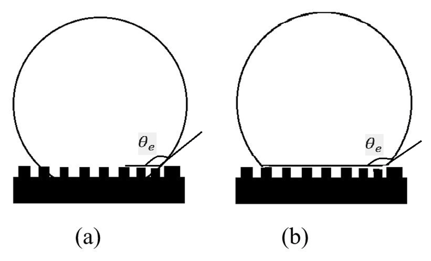
In the past, two types of states in modelling was considered for a droplet in force equilibrium on a surface, i.e., Wenzel [39] and Cassie-Baxter [40] models. In WenzelŌĆÖs model, the droplet the liquid droplet conforms to the base surface with the inclusion of the surface roughness (See Fig. 1a). Wenzel proposed a modified equation of Young which is given by, cos(╬Ėw) = r cos(╬Ėe), where ╬Ėw represents the apparent ╬Ės on the wetted surface and r is the roughness factor or a ratio of the actual area to the projected area. The equation of Young is stated as, cos(╬Ėe) = (╬│SV ŌłÆ ╬│SL)/╬│LV, where ╬│ refers to the interfacial surface tensions with S, L and V as solid, liquid, and gas, respectively. In Cassie-BaxterŌĆÖs model, the liquid droplet retains an almost spherical or round shape on the rough structure surfaces without conforming the base surface (See Fig. 1b). The Cassie model is expressed by, cos(╬Ėc) = f cos(╬Ėe) ŌłÆ (1 ŌłÆ f), where ╬Ėc represents the apparent ╬Ės on the composite surface and f is the area fraction of the solid surface in contact with the liquid. The Cassie-BaxterŌĆÖs model is associated with high apparent ╬Ės. It showed a lesser hysteresis ╬Ės than WenzelŌĆÖs model [41ŌĆō47]. WenzelŌĆÖs state predicts a ŌĆ£stickyŌĆØ surface. Cassie-Baxter-type surfaces predict a ŌĆ£slipŌĆØ surface. Generally, a droplet has more resistance to move on a ŌĆ£stickyŌĆØ than a ŌĆ£slipŌĆØ surface.
According to Patankar [48], the droplet can have two distinct contact angles on the same rough surface. The droplet can rest in a stable position of WenzelŌĆÖs state or Cassie-BaxterŌĆÖs state that oneŌĆÖs ╬Ės is higher than another. There is no guarantee that the droplet will always go to its lowest energy state (WenzelŌĆÖs state) from the higher energy state (Cassie-BaxterŌĆÖs state). Later, He et al. [47] confirmed the prediction through experiments. However, the exact details of the transition are not well understood. Patankar [48] believed that intermediate energy barrier exists. For droplet to be in the lowest energy state, the liquid must start filling the valleys or grooves of the substrate as the transition occurs. Another method is to press the droplet down to enable transition [49].
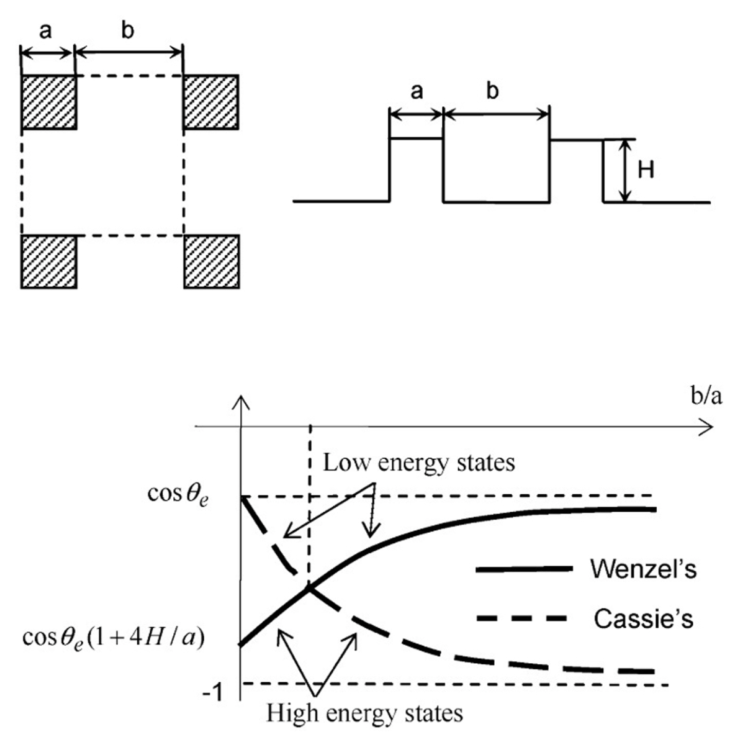
In applying the theories, He et al. [47] created a composite surface consisting of different materials. Droplet on the top surface of pillars has a different ╬Ės than the droplet conforming the base surface. Then, He et al. [47] varied the spacing of the pillars to achieve a robust superhydrophobic surface which consists of a common state surface energy for the droplet. He et al. [47] applied the equations of states (WenzelŌĆÖs state and Cassie-BaxterŌĆÖs state) and related the constants with the pillar spacing. As shown in Fig. 2, a unit cell of pillar with ŌĆśaŌĆÖ as the side and ŌĆśbŌĆÖ as the spacing between two pillars. The WenzelŌĆÖs state equation is given as,
cos ( ╬Ė w ) = [ 1 + 4 A ( a / H ) ] cos ( ╬Ė e )
3.2 Different hydrophobicity in applications
In air conditioning systems, aluminium fins of an evaporator use the hydrophilic coating for preventing the droplet from bridging between the fins [12,50ŌĆō52]. In the condensates formation study, it uses a hydrophilic surface for observing the dynamics coalescences with the neighbouring condensates [53ŌĆō55]. Such study helps to develop a more efficient way of removing condensates from fin surfaces [27ŌĆō30]. For hydrophobic surface, the applications are, e.g., anti-icing surface [56ŌĆō60], droplet impact on hydrophobic surface [61ŌĆō63], microliter droplet evaporation [64ŌĆō66], nanoliter droplet dispensers [67ŌĆō69], droplet sliding behaviour on different surface roughness [70ŌĆō72] and different surface structures [73ŌĆō75]. The applications of superhydrophobic surface are similar to hydrophobic surface ones, e.g., anti-freezing [76ŌĆō78], condenser/evaporator [78ŌĆō80] and microfluidic valves [81ŌĆō83]. The methods of fabricating superhydrophobic surface are the solidification of melted Alkylketene-dimer [84ŌĆō86], anodic oxidisation of aluminium [87ŌĆō89] and microwave plasmaenhanced CVD method using Trimethylmethoxysilane (TMMOS) [90ŌĆō92]. In nature, raindrops slide down on lotus leaves in a superhydrophobic condition [93ŌĆō95]. It gathers dust particles which result in a self-cleaning in the process of rolling down. In actual, the droplet rests or move with a short contact length on the superhydrophobic surface, which creates very little resistance for the droplet to slide down [23,36,96].
Mixed surfaces can be a patterned surface of hydrophilic/hydrophobic stripes. It is studied for a passive control system on droplets sliding down motion [97ŌĆō99]. Lee et al. [22] studied the sliding direction of droplet changes with different orientation of stripe-patterned surfaces using computational modelling. In microfluidics application, a sliding mechanism or gravity-induced method generates high quantity droplets in nanoliter size on patterned hydrophilic dots on the hydrophobic surface [100ŌĆō102]. On the other hand, Yong et al. [23] showed that the droplet accelerates on the hydrophilic surface in the cavity when sliding down from a hydrophobic surface. As shown in Fig. 3, it consists of the all-hydrophobic surface geometry (Fig. 3a) and the geometry of mixed surfaces (Fig. 3b). To be specific, the geometry of mixed surfaces consists of the hydrophobic top surfaces and the hydrophilic surfaces in the cavity. In Fig. 3b, the droplet moves filled in two cavities in inline. It is faster than the condition in Fig. 3a comparatively. This finding showed that a sudden change in the ╬Ės in the specific order of, lower surface energy (i.e. hydrophobic surface) to the higher surface energy (i.e. hydrophilic surface), had enhanced the droplet mobility. In the conservation law of energy, the potential energy stored in the droplet surface tension was released or converted into kinetic energy as the ╬Ės changes from a higher ╬Ės to a lower one in the cavity [103].
3.3 Droplet sliding down on surfaces
A droplet retained on a tilted surface exhibits variations in ╬Ės azimuthally. Parameters such as ╬Ės hysteresis, the difference between its advancing angle (most significant ╬Ės) and receding angle (smallest ╬Ės), are introduced to characterise their relation at inclined plane [104ŌĆō106]. The ╬Ės hysteresis for a droplet on polymer surface does not mean simultaneously equal to the surface inclination at which it started to slide downward [71,107]. It implies that the relation of ╬Ės hysteresis and gravitational pull is a non-linear one. Another method of studying the advancing and receding angle was done by spreading and slurping the water droplet from its source [72].
On tilted surfaces, the droplet slide down with (i) rotating motion on a hydrophilic surface, (ii) partially rotating and slip-off motion on the hydrophobic surface, (iii) a full slip-off motion on the superhydrophobic surface [36]. Recently, Yong et al. [23] validated the CFD results of droplet sliding down on a surface for cases of the hydrophilic (╬Ės = 79.2) and the hydrophobic (╬Ės = 98.7┬░) conditions. The comparisons used the experimental results of Sakai et al. [36]. The water droplet was 30 ╬╝L, and the slope or the tilted angle was 35┬░. As shown in Fig. 4a, the case of a hydrophilic condition that used the setting of ŌĆśno-slip wallŌĆÖ was the closest result with a difference of 5% only. For the case of hydrophobic condition (See Fig. 4b), it used the setting of ŌĆśslip-wallŌĆÖ which had the closest result as compared to SakaiŌĆÖs experimental result. However, the velocity profiles of Fig. 4b was about 7 to 10 times higher as compared to the work of Suzuki et al. [70]. The water droplet was experiencing a cyclic motion of elongation and contraction when sliding down the plane with the hydrophobic condition (╬Ės = 105┬░). The difference in the surface roughness (e) caused the discrepancies. Suzuki et al.[70] used surface of, e = 4.6 nm while Sakai et al.[36] used a surface of, e = 0.19 nm. Generally, it indicated that the CFD model capable of predicting the motion of water droplet on a surface with roughness less than, e = 0.19nm.
3.4 Droplet detachment in a microchannel
The behaviour of droplet detachment in microchannel is subject to parameters like the channel size, hydrophobicity of the walls and GDL (uneven fibre features [8]), droplet generation rate, the pressure difference, temperature changes, the permeability of the GDL and electric current flow [5ŌĆō9]. Cho et al. [9] conducted experiments to model the droplet behaviour in a microchannel and obtained both the top and side views of a droplet in the experiment. Cho et al. [9] developed a coefficient of drag for a droplet in the microchannel and estimated the velocity and the droplet size that about to detach from its source. Then, Cho et al. [9] used these correlations and developed an estimation of the droplet shape and validated it using numerical solution.
Theodorakakos et al. [5] investigated a droplet behaviour on three different surfaces. The droplet remained the same shape in the steady flow condition but the ╬Ės would change with different temperature. The shape of the droplet was similar to the work of Hao & Cheng [7] who used LBM for the predictions. Also, they observed that the droplet detached from the wall only at a very high gas velocity (~16 m/s). However, the gas flow rate in the application is around 5 m/s or equal to Re 164 due to the practicality [8]. The droplet that is nearer to the sidewall tends to travel toward the side walls in the gas-flowed rectangular channel. It formed a water film on the wall as more droplet started to accumulate on it [8].
Zhu et al. [6] studied the motion of the droplet in a continuous generation. The modelling setup is much closer to the actual conditions. The continuous generation of droplet affects the motion of the previously detached droplet in the microchannel. As the droplet occupies the microchannel, the free-flow area becomes lesser. Thus, the flow pressure focus on the new droplet more than the previously detached one. The same approach was used in Qin et al. [8]. Zhu et al. [6] investigated the droplet behaviour in a rectangular microchannel of different aspect ratio (AR), of height to width, with the same cross-section area. The findings showed that the droplet tends to stick at side-walls for cases of high AR cases. On the other hand, the droplet tends to stick on the top wall for all cases of low AR. The longest detachment time and the largest detachment diameter occur in cases of AR of 0.5 unit. The longest removal time for a droplet to exit the microchannel occurs at AR of 0.25 unit. The highest pressure drop in the microchannel consisting a droplet occurs at AR of 0.1 unit. Also, a semi-circular microchannel was investigated as well. The detachment time for semi-circular channel is longer than the rectangle but the removal time is shorter than the rectangular cross-section type.
Furthermore, Zhu et al. [6] investigated other types of cross-section, i.e. the rectangular with the curved bottom wall, trapezoidal, upside-down Trapezoidal, triangular microchannels. Those microchannels have equal width and height. The constraints were practical as it would not change the number of channels per row in the arrays. They measured the detachment time, the droplet diameter during detachment and the total droplet removal time. The performance favoured the triangular cross-section; in descending order, it followed by a trapezoid, the rectangle with a curved bottom wall, rectangular, upside-down trapezoid. They presented the results in ratios, i.e. (i) the wetted area to the area of microchannel wall, (ii) the water volume to the microchannel volume and (iii) the friction factor during operation to friction factor of an empty microchannel.
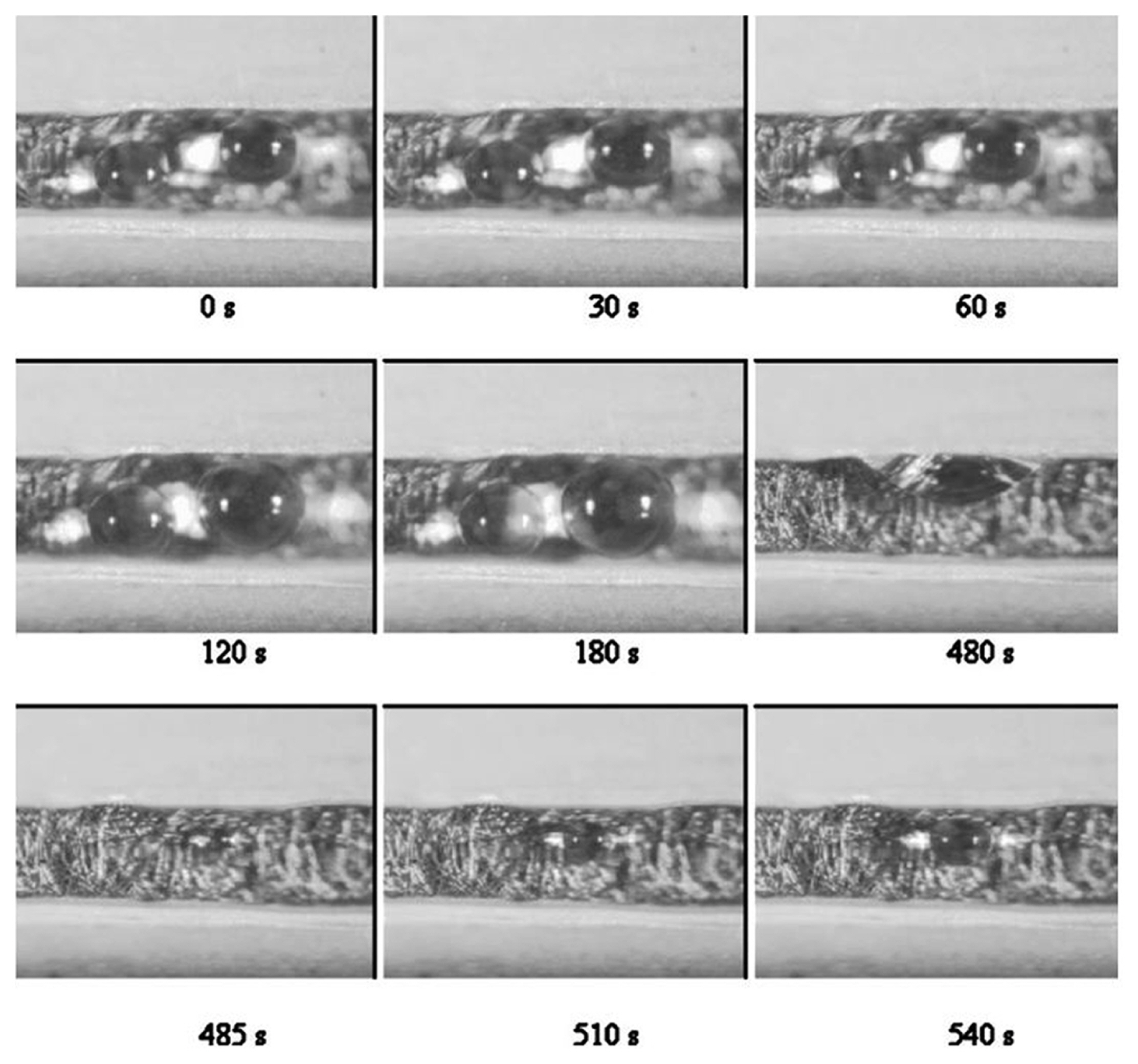
Yang et al. [108] observed the dynamic behaviour of water droplets in a gas microchannel. The setup characterised the test under automotive condition, i.e., 0.82 A/cm2 and 70┬░C. As shown in Fig. 5, two adjacent water droplets were growing next to each other. In the first 180s, those droplets were still growing in its initial position on the carbon paper. The ╬Ės of the droplets was between 70┬░ to 80┬░. The growth of the water droplet was found to be non-linear or discontinued at times. It happened when the water inside the GDL layers was still filling or spreading beneath it. At the time 480 s, droplets coalescence happened in the microchannel. It happened between two droplets that were growing closer together. As the droplets collide, it sticks to the hydrophilic wall on the side. In the authorsŌĆÖ opinion, the droplet could had experienced agitation on the liquid-vapour interface or a slight jump from the floor upon the coalescence (The phenomenon is described in Section 3.5).
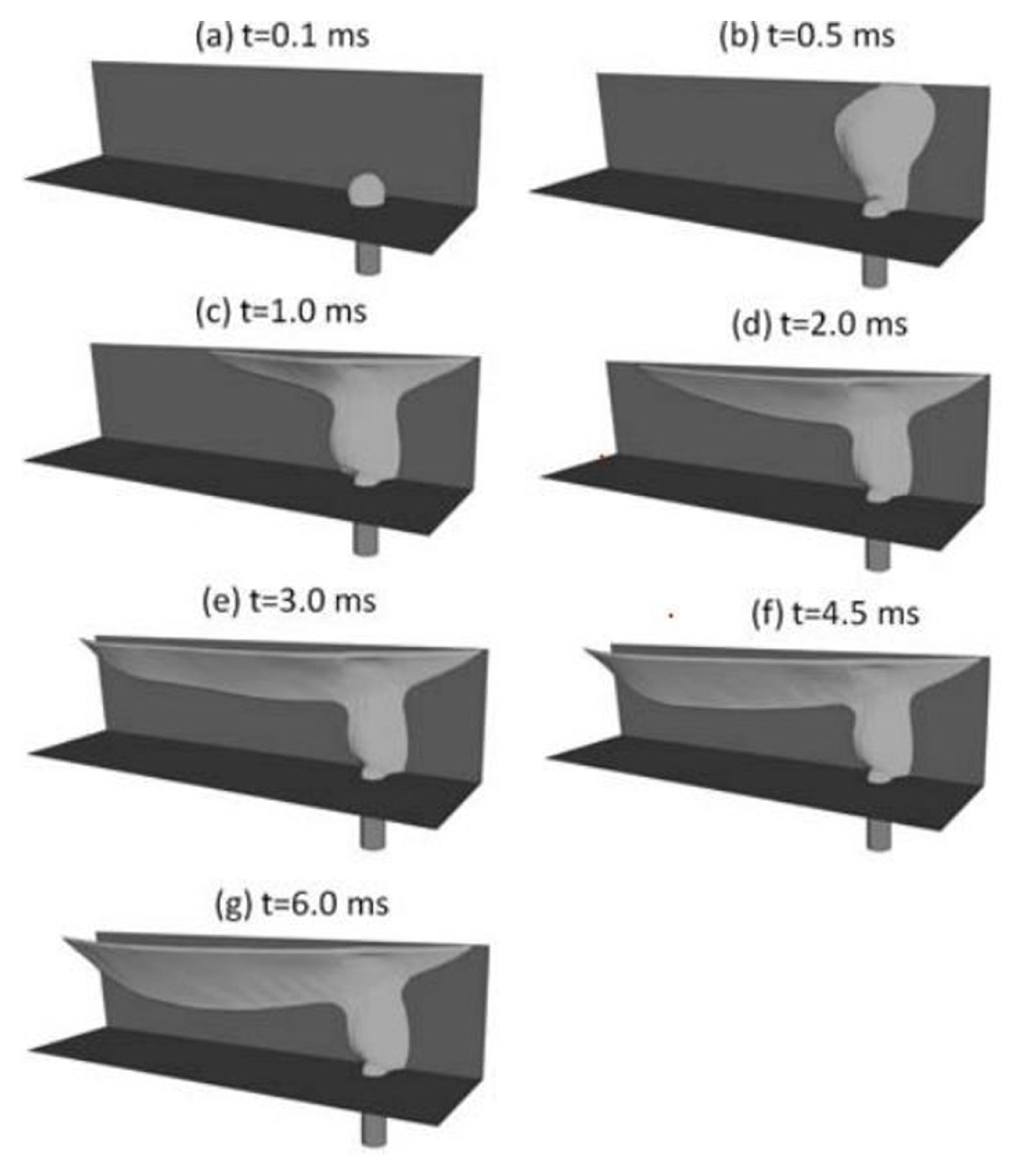
Qin et al. [8] investigated the phenomenon by performing a series of CFD simulations and focused on the role of walls hydrophobicity and the GDL for the water dispensing purpose. Qin et al. [8] found that the droplet took a shorter time to detach from the source than the surface of a higher hydrophobicity. During the detachment, the droplet leaned forward, and the ascending ╬Ės increases with higher gas flow rate. Furthermore, Qin et al. [8] confirmed that the microchannel walls in the hydrophilic conditions could prevent the microchannel from clogging. At first glance, those physical behaviours may seem to contradict the understanding that the droplet would travel faster on the hydrophobic surface (GDL). As shown in Fig. 6, Qin et al. [8] showed that the temporal result of transporting the volume of liquid on the sidewalls of a microchannel. Similar to the observations made by Yang et al. [108]sŌĆÖ experiment, the gas flow induces drag on the water film. Over the time, the film on the hydrophilic wall grew toward the end of the microchannel as the air-flow was shearing the film. Qin et al. [8] was able to observe the liquid film that was thinning at the leading edge but thickening at the end of the microchannel (exit). The airflow had caused the extra volume of water to propagate as surface wave toward the exit. As the water volume increases at the end of the channel (film), the liquid would sheared-off by the gas flow eventually.
3.5 Droplet jumping upon coalescence
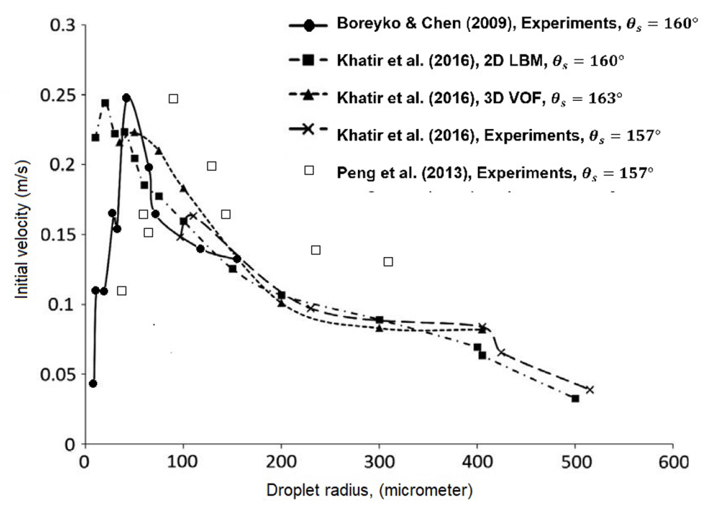
The droplet was found to jump spontaneously upon coalescence on the superhydrophobic surface [109ŌĆō112]. Boreyko and Chen [111] estimated the conversion for the jumping motion; it was about 20% of the total energy released upon the coalescence. For the same quantity, Peng et al. [109] estimated 25.2% of that total energy. Large droplet would jump with a lower velocity than the small droplet. However, the velocity of very tiny droplet limits by air resistance [111]. Therefore, an optimum condition exists for the droplet to jump at the highest velocity. Khatir et al. [29] investigated different droplet radius; ranging from 100 to 515 microns. As shown in Fig. 7, Khatir et al. [29] compared the numerical results of VOF and LBM and the experiments. Khatir et al. [29] estimated that the droplet with a radius of 35ŌĆō40 ╬╝m would jump at the highest velocity on a surface with ╬Ės = 160┬░. The peak condition of VOF results were closer to the experimental results of Boreyko and Chen [111] sŌĆÖ rather than Peng et al. [109]sŌĆÖ. Zhang & Yuan [113] demonstrated the effect of different surface roughness on the phenomenon. The surface condition that favour droplet jumping is the surface with roughness properties of the smaller skewness, the larger root mean square and Kurtosis of three units approximately. The predicted velocity is well within the prediction of Fig. 7. Generally, the condition of which the droplets jump with the highest velocity (in average) is thought to yield the highest rate of condensation. However, that assumption had excluded the effect of airflow on the trajectories of droplets and the heat transfer on the surface. Miljkovic et al. [110] investigated the effect of electric-field on the phenomenon under the influence of airflow. The significant insight were that the droplets were jumping with longer distances due to the enhancement of the electric field, and the small droplets were jumping at early coalescences. As compared to state-of-art dropwise condensation, Miljkovic et al. [110] reported that the electric-field enhanced the condensation and the overall heat transfer up to 30% and 50% respectively
4. Comparisons of the Selected Categories
In the current section and sub-sections, the ŌĆśType- AŌĆÖ simulation represents the computational modelling cases of droplet sliding down a surface. The ŌĆśType-BŌĆÖ simulation represents the computational modelling cases of droplet detachment in a gas-flowed microchannel for PEMFC application. The ŌĆśType-CŌĆÖ simulationŌĆÖ represents the computational modelling cases of droplet jumping upon coalescence on a superhydrophobic surface.
4.1 Publications
As shown in Fig. 8, there is a growing interest in computational modelling regarding the study of droplet sliding down a surface (Type-A) [14ŌĆō23]. As compared to other categories, the computational modelling of droplet detachment in a gas-flowed microchannel for PEMFC application (Type-B) has no updated publication since 2012. Recently, new modelling studies that are related to PEMFC technology are, i.e. the phenomenon of water droplet jump upon coalescence in microchannel [114], the water droplet breaking through a gas diffusion layer [115] and droplet sliding angle on hydrophobic wire screens [116]. In another category, the publication related to the phenomenon of droplet jumping upon coalescence on a superhydrophobic surface (Type-C) increased rapidly in recent years. Such a phenomenon could enhance the performance of condensation process for the ease of removing condensates from the fin surfaces [111].
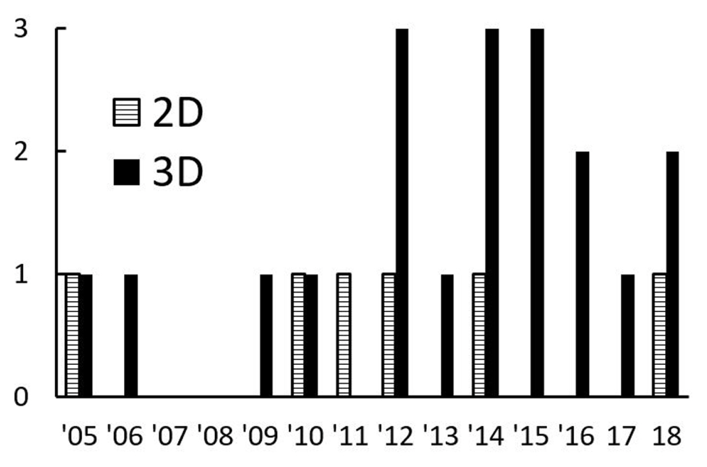
The present review finds that the publications with the three-dimensional (3D) modelling are higher in numbers than the two-dimensional (2D) ones. As shown in Fig. 9, the number of publications concerning 2D modelling was comparatively low ceased in 2014. Most of the 2D computational modelling was published with unique numerical approaches or techniques [14,17,18,30] and to validate the solutions [9]. Liu and Peng explained the limitation of using 2D computational modelling for droplet dynamics [24,26]. Recently, a new 3D front-tracking method that integrates the generalised Navier boundary condition to model the moving contact line had been developed to replace the previous 2D modelling method [117].
4.2 Hydrophobicity and droplet size
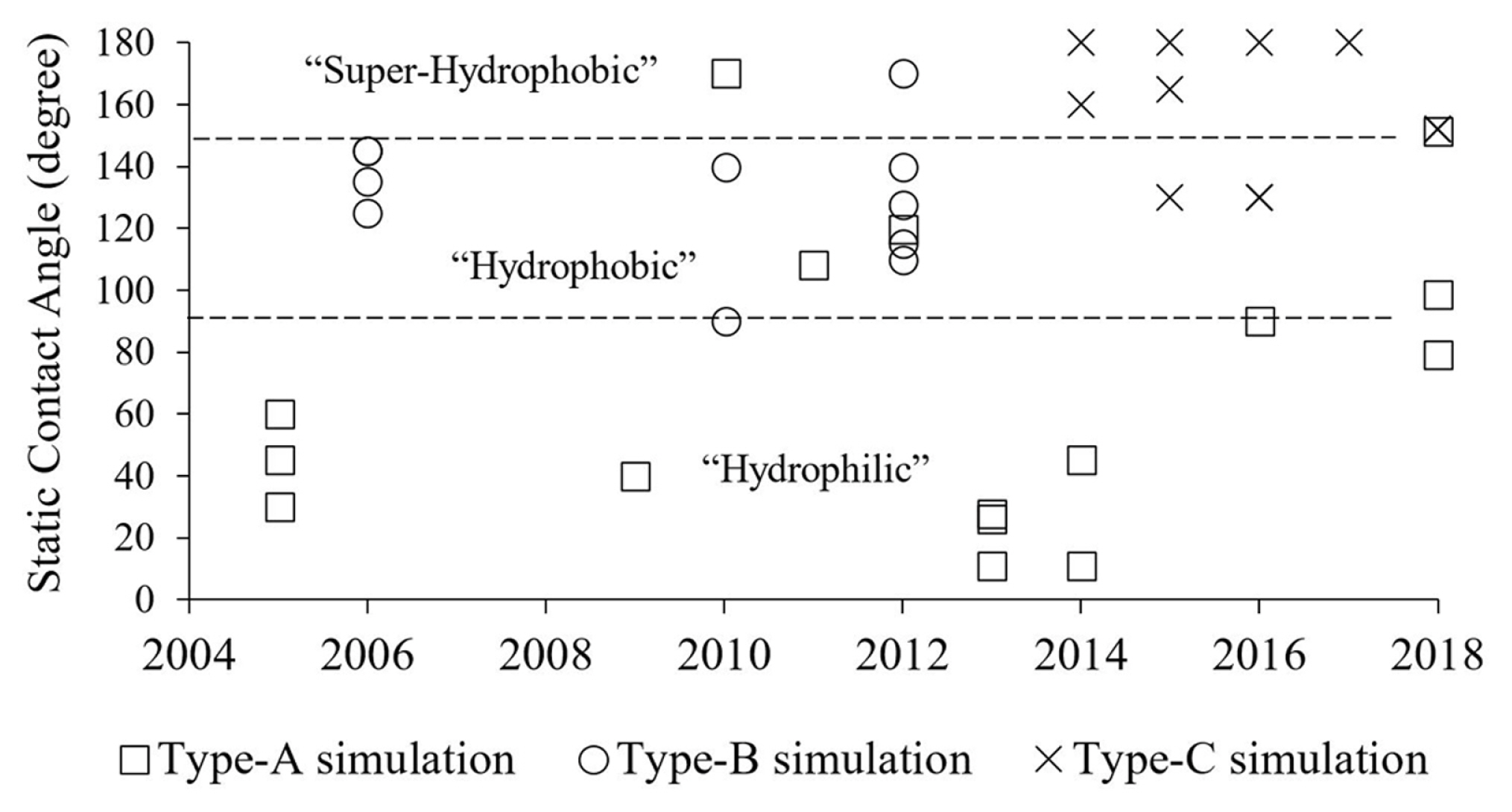
The natural hydrophobicity used in each category of the studies is noticeable. As shown in Fig. 10, the most investigated surface in the category of droplet sliding down a surface (type-A) was the hydrophilic type. A few studies were carried out on hydrophobic [18,19,23] and superhydrophobic condition [17]. The hydrophobic surface was used mainly in the category of droplet detachment in a gas-flowed microchannel (type-B). On the other hand, Theodorakakos et al. [5] and Qin et al. [8] extended the ╬Ės in the study to 160┬░ and 170┬░, respectively. The superhydrophobic surface was used mainly for the category of droplet jumping upon coalescence (type-C). In some studies, the ╬Ės was as low as 130┬░ [28ŌĆō30] and as high as 180┬░ [25,27,29].
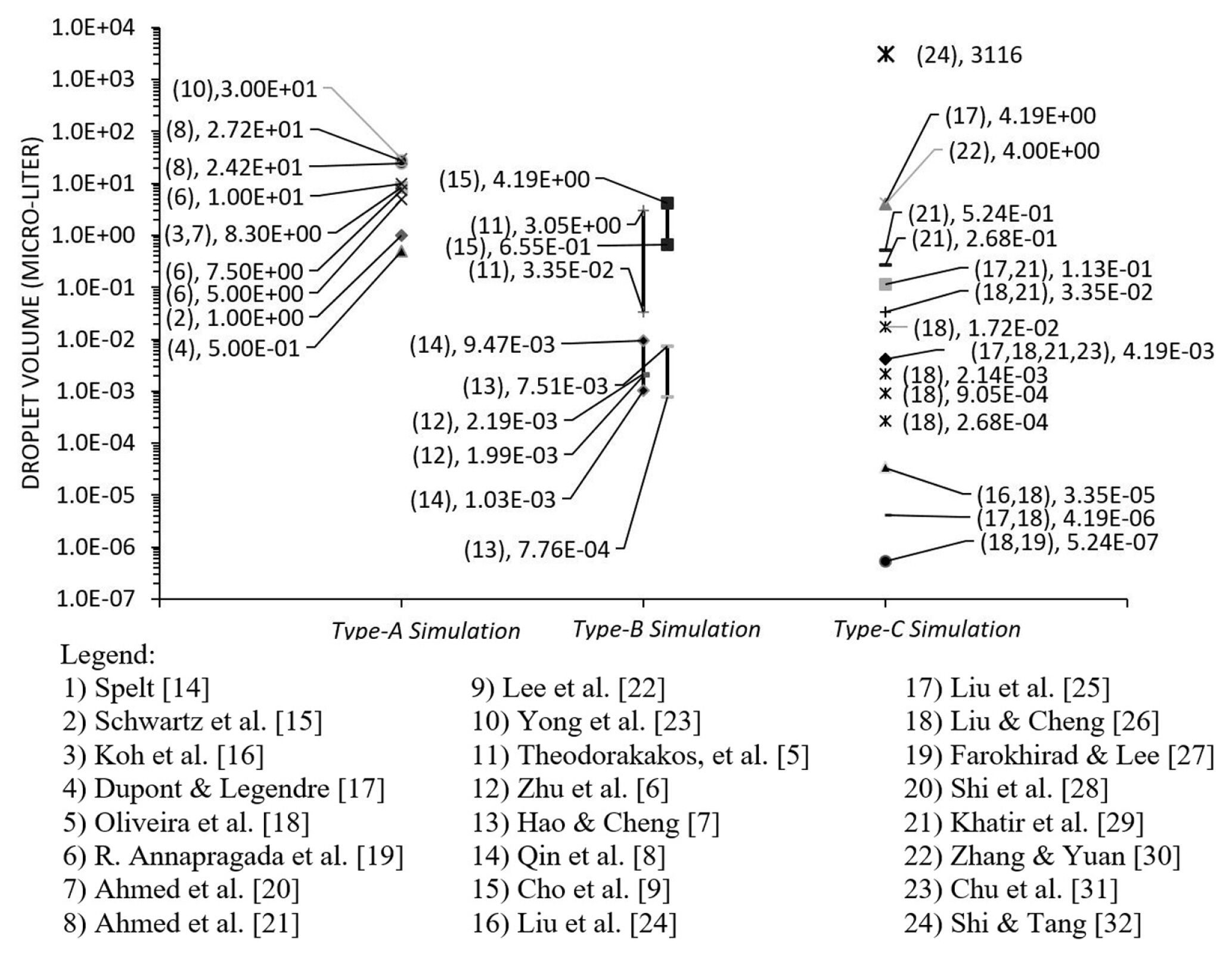
Liquid water is the commonly used fluid in computational modelling except for Ahmed et al. [20] who used PPG/Silica and Blood (non-Newtonian fluid) and Koh et al. [16] who used silicon oil properties. In Fig. 11, the droplet volume in the categories of type-A, type-B and type-C are grouped and presented with each volume (data point). As a note, the distribution had excluded the literature with dimensionless data. Generally, the droplet size used in Type-A simulation was the largest as compared to other categories. For type-B, the range of droplet size was between the Type-A and Type-C. The estimation of the droplet size in the microchannel was equal to the duration of detachment time multiplied by the rate of injection. Among the categories, ŌĆśType-CŌĆÖ simulation had the most extensive range of droplet size. It indicated that the factor of hydrophobicity influenced the phenomenon more than the size of the droplet itself [115].
4.3 Boundary conditions
In the category of droplet sliding down on a surface, the tilted angles commonly used in computational modelling were 30┬░, 45┬░ and 60┬░ [16,19ŌĆō21]. Other specific inclinations were 6┬░, 13┬░, 19┬░, 26┬░, 29┬░, 40┬░ and 79┬░ as found in the work of Dupont and Legendre [17]. The smallest tilted angle was 4.7┬░ [18]. In the past, computational modelling investigated the droplet sliding down behaviour on a vertical plane (90┬░) for the hydrophilic surface only [14,15]. In most of the computational modelling, it uses a plain surface with non-slip boundary condition. For non-plain surfaces, it was found mainly in the category of droplet jumping upon coalescence on a superhydrophobic surface (type-C), e.g. such as cavities, square pillars [24,26], conical pillars [28] and random structures [30]. In the Lattice Boltzmann method (LBM), the standard size of a square pillar shape was 2├Ś2 lattices, 16 lattices in height and with spacing varying from 4 to 28 lattices. For other categories, Oliveira et al. [18] used ramped pillars for the droplet to slide down (type-A).
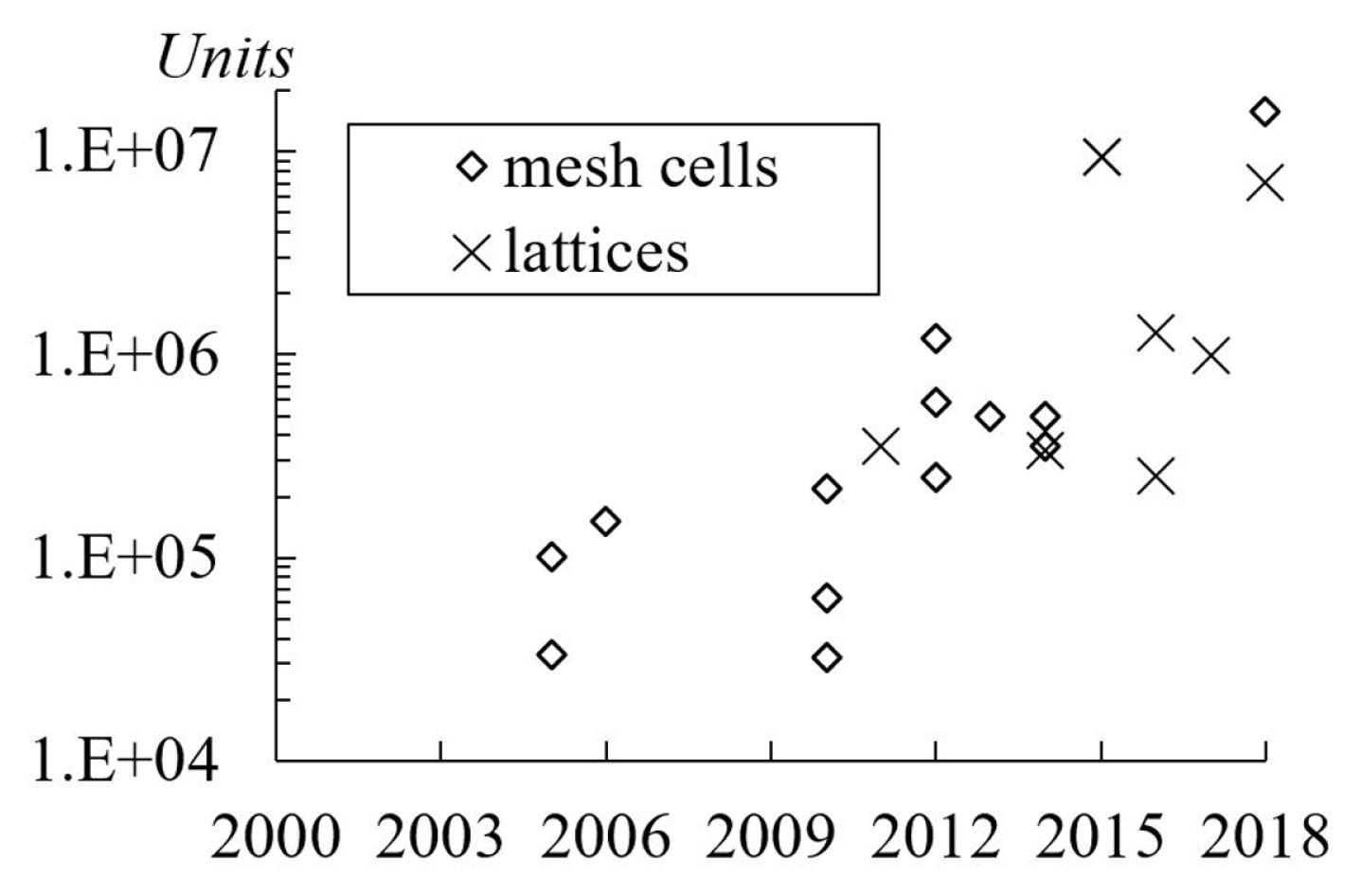
4.4 Mesh cells and computational domain
The average number of mesh cells used in the studies is approximately 500, 000 units [9,15,16,23]. In Fig. 12, it is notable that the total mesh cells or lattices used in simulations increase each year. As a note, the present review excluded the publication related to mesh independency study [33]. Another interpretation of mesh size is the number of cells per droplet radius. Typically, it was approximately 22 to 40 cells. The highest number of cells per radius was 100 units as applied by Schwartz et al. [32] who use ŌĆ£Longwave or lubrication approximationŌĆØ coupled with ŌĆ£disintegrated pressureŌĆØ. In the Lattice Boltzmann method, a lattice unit is a measurement unit for the computational domain size. Hao and Cheng [7] had used 60 lattices per radius. However, Farokhirad et al. [27] did a grid dependency study and concluded that the use of 25 lattices per radius was sufficiently accurate.
The computational domain shape in each type of simulation was unique to its application. For illustration, the present review uses cases of LBM. The computational domain of e.g. (i) droplet sliding down on a surface (type-A) category shaped like a flat plane with 40├Ś80├Ś80 lattices [22], (ii) the droplet detachment in a gas-flowed microchannel (type-B) category shaped like an elongated cube with 60 ├Ś30 ├Ś120 lattices [7]; the usual cross-section of microchannel is a quadrilateral shape, some are triangular shape with hydrophilic walls [118ŌĆō120], (iii) droplet jumping upon coalescence on superhydrophobic surface (Type-C) category shaped like tall cube with 192├Ś192├Ś256 lattices [28]. In type-B, the cross-section of the rectangular shape of the microchannel is the most common one. The standard aspect ratio was approximately two units in height to 1 unit in width [6ŌĆō9]. On the other hand, Zhu et al. [6] simulated various sizes of micro-channels with aspect ratios ranging from 1:10 to 2:1. The channel length was ranging from 0.5 mm [8] to 5 mm [5]. The gas flow rate in the channel could range up to Re 300. The microchannel with the lowest cross-section height was 0.079 mm with gas flow rates of 10m/s or equal to Re 90.
4.5 Numerical methods
The challenges in modelling droplet liquid-vapour interface include (i) implementing of mass and momentum conservation equations, (ii) modelling the discontinuities in fluids density across the interface and (iii) handling of complex numerical treatment for droplet advection. For modelling the physics, there are several numerical models, e.g. ŌĆ£long-wave or lubrication approximationŌĆØ coupled with the ŌĆ£disjoining pressureŌĆØ model [32] with the accuracy of this method being dependent on the sub-layer height in addition to the mesh size [16]; Volume- of-Fluid (VOF) with unique numerical treatments that track the droplet advection and free-surface interfaces [121]; and the LBM [7,122].
ŌĆ£Long-wave or lubrication approximationŌĆØ coupled with the ŌĆ£disjoining pressureŌĆØ model assumes a layer of liquid with an isolated droplet on a plane substrate. The liquid surface corresponds to z = h(x, y, t) where t is time. The mass conservation, ht = ŌłÆ┬ĘŌłć┬ĘQ + wi(x, y, t), where wi is a local injection rate and the term,
Q = Ōł½ 0 h ( x , y ) ( U , V ) d z
In the VOF method, a sharp interface is commonly used to represent the liquid-vapour interface for the one-fluid and two-fluid models [19,21]. The approach volume fractions of liquid-solid regions embedded the geometry into the mesh. In the VOF method, the mass continuity equation is
whereVF is fract ional volume open to flow, (Ax,Ay,Az) are the fractional areas that open to flow. The parameter Žü is the fluid density, and the variables (u, v, w) are the fluid velocity components. It uses the fractional face areas and the fractional volumes of the cells that are open to the flow for defining the wall boundary features in the mesh. In each cell, the solver computes the surface fluxes, surface stress, and body forces. It treats the cell as a control volume. These quantities are then used to form approximations for the conservations laws as expressed by the equation of motion. The equations of motion for the fluid velocity components are the Navier-stokes equations as given in the following
where (Gx,Gy,Gz) are the body accelerations and (fx,fy,fz) are the fluid accelerations. In the present study, the explicit solver solves the viscous stress, surface tension pressure, and advection motion. It evaluates the equations using the current time-level values of the local variables.
On the other hand, it solves the local pressures and velocities, which are coupled implicitly, by using the time-advanced pressures in the momentum equations and time-advanced velocities in the mass (continuity) equation. This semi-implicit formulation, however, results in coupled sets of equations that must be solved by iterative techniques which include the generalised minimal residual method (GMRES). The approximation for the volume of fluid function (free surface) in Eulerian grids is
where F is scalar,
(4)
ŌĆśhŌĆÖ is the height of fluid in the cell. The advection of the free-surface is done using three steps [124]. The first step is to approximate the fluid interface in a unit mesh with a planar surface. The second step is to approximate the fluid volume movement according to the local velocity field. For example, the distance dx in the x-direction is computed using a second-order integration for equation as follows:
The third step is to compute new fluid fraction values in the computational mesh using an overlay procedure where an adjustment of the computed fluid volume. The procedure makes sure that the combined volume of fluid in the acceptor unit meshes is made equal to the volume in the donor unit mesh [121,124].
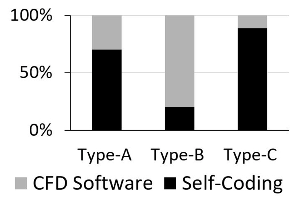
As shown in Fig. 13, most of the publications regarding droplet sliding down on a surface (type-A) were performed by numerical ŌĆśself-codingŌĆÖ while the remaining percentage used CFD software. In that regard, the ŌĆ£long wave or lubrication approximationŌĆØ coupled with ŌĆ£disintegrated pressureŌĆØ [15] was the most-used and effective method for modelling the 3D droplet movement on a hydrophilic surface. The same method was applied by Ahmed et al. [21] for non-Newtonian droplets such as blood and PPG silica solutions in the modelling of the droplet spread on an inclined surface. Other numerical ŌĆ£self-codingŌĆØ are LBM [122], the Level Set [14] and the Cellular Potts Hamiltonian [18]. In modelling droplet sliding behaviour at higher hydrophobicity, the preferred approach is the VOF method. For example, Dupont and Legendre [17] worked on modelling for droplet sliding on superhydrophobic with ╬Ės=170┬░ using VOF method of JADIM, while Annapragada et al. [35] modelled droplet sliding in a moving reference frame (a steady-state condition) on an inclined plane with ╬Ės = 120┬░ using the VOF method of FLUENT software. On the other hand, Yong et al. [23] modelled droplet sliding with advection in the computational domain for ╬Ės = 79.2┬░ and 98.7┬░ using VOF method of Flow-3D software.
LBM solves the discrete Boltzmann equation to simulate the flow with collision models. The Boltzmann equation is also known as the Boltzmann transport equation. It describes the statistical distribution of particles in a fluid. It is an equation for the time evolution where the particle distribution function in the phase space. The Boltzmann equation treats every stationary point in a computational domain that stores information. It stores information like its position, (x,y,z) in coordinates and momentums, (px,py,pz ). As such, the computational domain is known as a phase space, which has six dimensions since every variable is independent of one to another. Each point has the vector notation of (r,p) which is equal to (x,y,z,px, py, pz) .The vector parameter p is also known as ŌĆśmomentaŌĆÖ. In the computational domain, the discretised space element is written as (dxdydz┬Ędpxdpydpz) or (d3r┬Ę d3p). Supposedly, particles or molecules passing through a region in the computational domain over some time (t). The probability density function of the particles passing through the region is f(r,p,t) which is per unit phase-space. The function of the distribution gives the probability of finding a particular molecule for a given position and momentum [125]. The discretised count of the number of particles are, dN = f(r, p, t)d3r┬Ęd3p. The total number of particles in that region is stated as, N = ŌłŁ ┬Ę ŌłŁ f(x,y,z, px,py,pz, t)┬Ędxdydz ┬Ędpxdpydpz. The collision between particles is defined as the rate of change of forces, it is denoted as Ōłéf/Ōłét. The classic continuum Boltzmann equation for a single particle distribution function and written as, Ōłéf Ōüä Ōłét+c(Ōłéf Ōüä Ōłér)+ F Ōłéf Ōüä Ōłéc = Q(f) , where c is velocity as derived from p, F is the body force and Q( f ) is the collision integral. One of the major problem with LBM is to resolve the collision integral. As proposed by He and Luo [126], a straightforward expression that is the lattice Boltzmann with Bhatnagar- Gross-Krook (BGK) approximation or singlerelaxat ion-time model and is given by, QBGK(f) = ŌłÆ(f ŌłÆ feq)/Žä, replaces the collision integral. The parameter Žä is a typical single-relaxation-time associated with collision relaxation to the local equilibrium. In the present review, the LBM of isothermal and hydro-dynamics often use three dimensional and 19 velocity lattice (D3Q19) stencils with the multi-relaxation-time (MRT) approach as it has higher numerical stability than that of the single-relaxation- time approach. The evolution equation with MRT collision operator is given by,
f ╬▒ ( X + e a ╬┤ t , t + ╬┤ t ) = f ╬▒ ( X , t ) - ╬Ż ╬▓ ╬® ╬▒ ╬▓ ( f ╬▓ ( X , t ) - f ╬▓ e q ŌĆē ( X , t ) ) + S ╬▒ ( X , t ) - 0.5 ╬Ż ╬® ╬▒ ╬▓ S ╬▓ ( X , t ) f ╬▓ e q
Generally, the computational modelling of droplet detachment in a gas-flowed microchannel (type-B) is more complicated. It is a multiphase flow computational modelling where the droplet moves in the microchannel due to the shear and form drag brought on by the difference in gas pressure. In most cases, the small physical assembly itself limits the observation made on the droplet, especially from the side view and walls. For solution, CFD simulation was used to overcome the difficulty in measuring the ╬Ės on the walls and GDL layer [5]. In Fig. 13, most of the studies in that category were done using CFD software instead of ŌĆ£self-codingŌĆØ. For example, Zhu et al.[6], Qin et al. [8] and Cho et al. [9] used second-order schemes of FLUENT, while Theodorakakos et al. [5] used in-house VOF software in Eulerian grids and RANS models. On the other hand, in the numerical ŌĆ£self-codingŌĆØ method, limitations were found in the LBM in modelling the droplet in such conditions. The assumption the dynamic viscosity ratio of liquid and vapour are made the same. As such, it constrained the modelling to exhibit high fluidity with high-density ratio [7]. Later, Li et al. [127] proposed a forcing scheme of Multi-Relaxation-Time (MRT) pseudo-potential of LBM, which enables the method to solve with accuracy for density ratio around 500 times. However, it has yet to reach 1000 times to represent the density ratio of water to air. For the category of droplet jumping upon coalescence on a superhydrophobic surface (type-C), most of the previous studies performed numerical ŌĆśself-codingŌĆÖ. Liu and Peng [26] and Shi et al. [28], who adopted the pseudopotential LBM coupled with MRT collision operator, were able to model the phenomenon, while Farokhirad et al. [27] used LBM with Cahn-Hilliard diffuse interface theory for simulation of large density ratio. Despite these developments, numerical instability in LBM simulation was still highlighted [26,28].
4.6 Validations
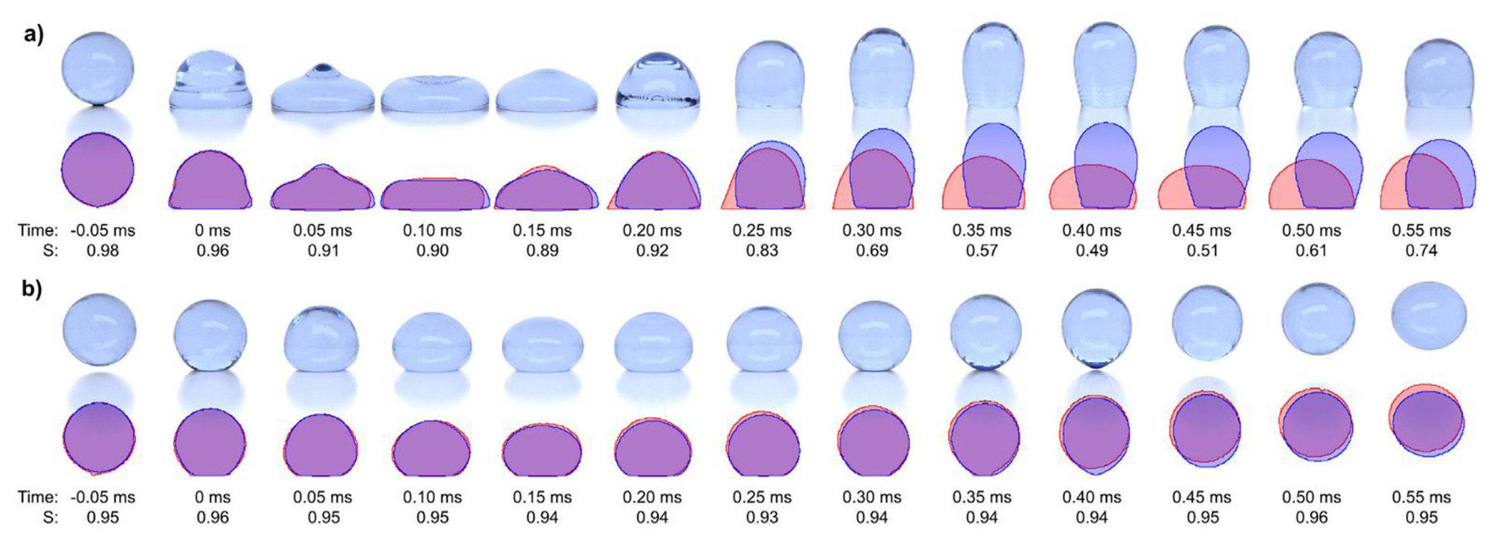
In validating the computational modelling of droplet sliding down a plane, Spelt [14] validated their numerical scheme of Level Set method with the boundary element method of Schleizer and Bonnecaze [128]. Besides other references [36,128ŌĆō130], Podgorski et al. [131]sŌĆÖ experimental results were the most preferred one for validating computational modelling results in that category [15,16,21]. Experimentally validated computational modelling results on droplet dynamics behaviour are crucial for further investigation in engineering and applications. Recently, Yong et al. [23] validated the CFD results of droplet sliding down on hydrophilic and hydrophobic surfaces. For superhydrophobic surfaces, the concerned type of simulation work with experimental validation is lacking in the publications. In reality, the droplet rests or move with a short contact length on the superhydrophobic surface, which creates very little resistance for the droplet to slide down. In the literature, most of the modelling assumed that the droplet has a full-surface contact with its base. As such, the modelling would have significant discrepancies with the experimental results. The discrepancy was observed in the validation work of Kulju et al. [132]. As shown in Fig. 14, the images compare CFD results of a droplet impacting on (a) a hydrophobic surface and (b) a superhydrophobic surface with the actual results. As compared to the CFD result of the superhydrophobic surface, the CFD result of the droplet impacting on a hydrophobic surface was inaccurate due to longer contact time. Since the ╬Ės is lower for a hydrophobic surface, the surface tension is lower as compared to a superhydrophobic surface. It bounced off with longer contact time. Simultaneously, it occupied a larger area, of which, it was a full-contact length. Thus, it reduced the kinetic energy of the droplet. In the case of droplet jumping upon coalescence on superhydrophobic surface, the experimental results of Boreyko and Chen [111] and the numerical work of Liu et al. [25], who used the pseudopotential model of LBM of Yue et al. [133], were the most popular reference for validation besides other references [110,134ŌĆō136]. In topics related to droplet detachment in microchannel [137ŌĆō139], most of the research works conducted own experimental works and performed numerical simulations [5ŌĆō7,9] except Qin et al. [8], who compared their computational modelling results with the experimental results of Bazylak et al. [10] and Hartnig et al. [12].
5. Conclusions
This paper reviewed three different types of droplet behaviours in particular related to the computational modelling and the water dispensing technology in PEMFC. The subject of droplet sliding down behaviour on surfaces showed that the significance of hydrophobicity and gravity force on the droplet motion. It serves as a useful reference for computational modelling study which uses more complicated body forces. The review found that the topics related to the performance or evaluation criteria for the microchannel shapes and design are still lacking in publications. Also, the present review anticipated that the future publication related to droplet dynamics behaviour in PEMFC would include more operational factors.